mygrad.nnet.layers.conv_nd

mygrad.nnet.layers.conv_nd(x: ArrayLike, filter_bank: ArrayLike, *, stride: Union[int, Tuple[int, ...]], padding: Union[int, Tuple[int, ...]] = 0, dilation: Union[int, Tuple[int, ...]] = 1, constant: Optional[bool] = None) → Tensor

Use filter_bank (w) to perform strided N-dimensional neural network-style convolutions (see Notes) over x.:

f(x, w) -> x ⋆ w

shapes:
(N, C, X0, ...) ⋆ (F, C, W0, ...) -> (N, F, G0, ...)

x represents a batch of data over which the filters are convolved. Specifically, it must be a tensor of shape \((N, C, X_0, ...)\), where \(N\) is the number of samples in the batch, C is the channel-depth of each datum, and \((X_0, ...)\) are the dimensions over which the filters are convolved. Accordingly, each filter must have a channel depth of \(C\).

Thus convolving \(F\) filters, each with a shape \((C, W_0, ...)\), over the data batch will produce a tensor of shape \((N, F, G_0, ...)\), where \((G_0, ...)\) is the shape of the grid commensurate with the filter placements

Parameters

xArrayLike, shape=(N, C, Xo, …)

The data batch to be convolved over.

filter_bankUnion[Tensor, array_like], shape=(F, C, Wo, …)

The filters used to perform the convolutions.

strideUnion[int, Tuple[int, …]]

(keyword-only argument) The step-size with which each filter is placed along the H and W axes during the convolution. The tuple indicates (stride-0, …). If a single integer is provided, this stride is used for all convolved dimensions

paddingUnion[int, Tuple[int, …]]

(keyword-only argument) The number of zeros to be padded to both ends of each convolved dimension, respectively. If a single integer is provided, this padding is used for all of the convolved axes

dilationUnion[int, Tuple[int, …]], optional (default=1)

(keyword-only argument) The spacing used when placing kernel elements along the data. E.g. for a 1D convolution the ith placement of the kernel multiplied against the dilated-window: x[:, :, i*s:(i*s + w*d):d], where s is the stride, w is the kernel-size, and d is the dilation factor.

If a single integer is provided, that dilation value is used for all of the convolved axes

constantOptional[None]

If True, the resulting Tensor is a constant.

Returns

Tensor, shape=(N, F, G0, …)

The result of each filter being convolved over each datum in the batch.

Notes

• The filters are not flipped by this operation, meaning that an auto-correlation is being performed rather than a true convolution.

• Only ‘valid’ filter placements – where the filters overlap completely with the (padded) data – are permitted.

Examples

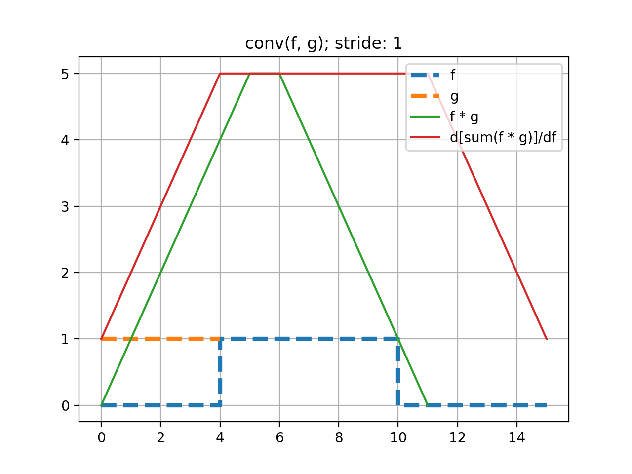
Here we perform a 1D convolution of a constant-valued kernel, k, with a ‘square-wave’ signal, x, using stride-1. Note that because we are constrained to doing deep learning-style convolutions, that we prepend the dimensions \((N=1, C=1)\) to x, and \((F=1, C=1)\) and to k. That is, we are performing a convolution on one, single-channeled signal using one kernel.

See that this convolution produces the expected triangle-shaped response. The shape of the resulting tensor is \((N=1, F=1, G_0=12)\). That is, the length-5 kernel can be placed in 12 valid positions, using a stride of 1.

>>> import mygrad as mg
>>> from mygrad.nnet import conv_nd
>>> x = mg.zeros((1, 1, 16))  # a square-wave signal
>>> x[..., 5:11] = 1
>>> k = mg.ones((1, 1, 5))    # a constant-valued kernel
>>> conv_nd(x, k, stride=1)   # performing a stride-1, 1D convolution
Tensor([[[0., 1., 2., 3., 4., 5., 5., 4., 3., 2., 1., 0.]]], dtype=float32)

Back-propagating through the (summed) convolution:

>>> conv_nd(x, k, stride=1).sum().backward()  # sum to a scalar to perform back-prop
>>> x.grad  # d(summed_conv)/dx
array([[[1., 2., 3., 4., 5., 5., 5., 5., 5., 5., 5., 5., 4., 3., 2., 1.]]],
      dtype=float32)
>>> k.grad  # d(summed_conv)/dk
array([[[6., 6., 6., 6., 6.]]])

(Source code, png, hires.png, pdf)

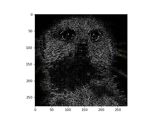
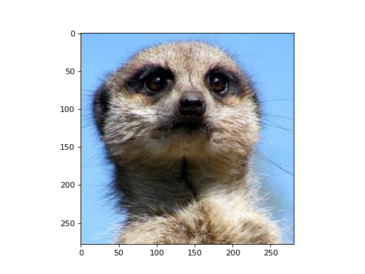
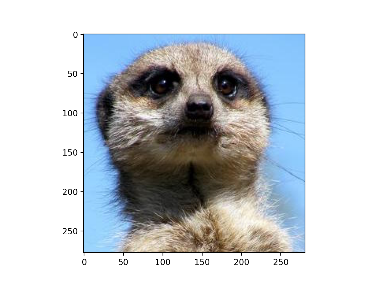
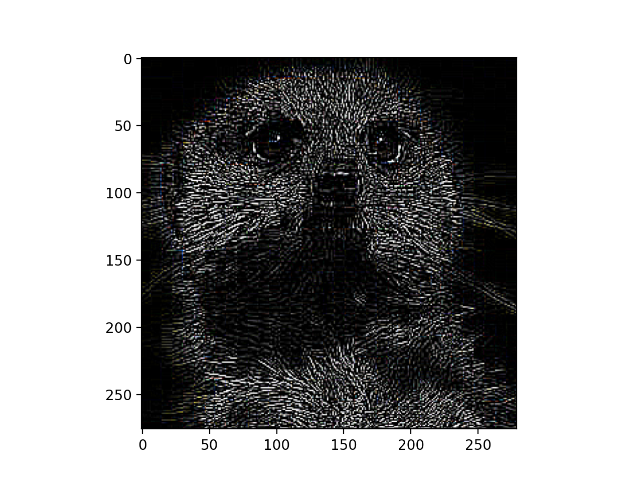
Let’s apply a edge-detection kernel to each color channel of an RGB image.

>>> import matplotlib.pyplot as plt
>>> import matplotlib.image as mpimg
>>> from mygrad.nnet.layers import conv_nd
>>> # A shape-(H, W, 3) RGB image
>>> img = mpimg.imread('../_static/meerkat.png')
>>> # We'll treat this like a batch of three greyscale images
>>> # where each "image" is actually a color channel
>>> # shape-(H, W, 3) -> shape-(3, 1, H, W)
>>> x = img.transpose(2, 0, 1)[:, None, :, :]

>>> # edge detection kernel
>>> kernel = np.array([[-1, -1, -1],
...                    [-1,  8, -1],
...                    [-1, -1, -1]])
>>> # (Hf, Wf) --> (1, 1, Hf, Wf)
>>> kernel = kernel.reshape(1, 1, *kernel.shape)

>>> # conv: (3, 1, H, W) w/ (1, 1, Hf, Wf) --> (3, 1, H', W')
>>> # squeeze + transpose: (3, 1, H', W') --> (H', W', 3)
>>> processed = conv_nd(x, kernel, stride=(1, 1))
>>> processed = processed.data.squeeze().transpose(1, 2, 0)

>>> fig, ax = plt.subplots()
>>> ax.imshow(img)

>>> fig, ax = plt.subplots()
>>> ax.imshow(processed)

(Source code)

(png, hires.png, pdf)

(png, hires.png, pdf)

Now, let’s demonstrate a more typical usage for conv_nd in the context of neural networks. x will represent 10, 32x32 RGB images, and we will use 5 distinct 2x2 kernels to convolve over each of these images . Note that each kernel must possess 3-channel - one for each RGB channel.

That is, we will be performing NxF channel-wise 2D convolutions. Supposing that we don’t want the kernel placements to overlap, we can use a stride of 2. In total, this will produce a shape-\((N=10, F=5, G_0=16, G_1=16)\) tensor as a result.

>>> import mygrad as mg
>>> x = mg.random.rand(10, 3, 32, 32))  # creating 10 random 32x32 RGB images
>>> k = mg.random.rand(5, 3, 2, 2))     # creating 5 random 3-channel 2x2 kernels

Given the shapes of x and k, conv_nd automatically executes a 2D convolution:

>>> conv_nd(x, k, stride=2).shape
(10, 5, 16, 16)

Extrapolating further, conv_nd is capable of performing ND convolutions!

Performing a convolution over a batch of single-channel, “spatial-3D” tensor data:

>>> # shape-(N=1, C=1, X=10, Y=12, Z=10)
>>> x = mg.random.rand(1, 1, 10, 12, 10)
>>> # shape-(F=2, C=1, Wx=3, Wy=1, Wz=2)
>>> k = mg.random.rand(2, 1, 3, 1, 32)
>>> conv_nd(x, k, stride=1).shape
(1, 2, 8, 12, 9)